pacman::p_load(igraph, tidygraph, ggraph,
               visNetwork, lubridate, clock,
tidyverse, graphlayouts)Hands-On_Ex05
GAStech_nodes <- read_csv("data/GAStech_email_node.csv")Rows: 54 Columns: 4
── Column specification ────────────────────────────────────────────────────────
Delimiter: ","
chr (3): label, Department, Title
dbl (1): id
ℹ Use `spec()` to retrieve the full column specification for this data.
ℹ Specify the column types or set `show_col_types = FALSE` to quiet this message.GAStech_edges <- read_csv("data/GAStech_email_edge-v2.csv")Rows: 9063 Columns: 8
── Column specification ────────────────────────────────────────────────────────
Delimiter: ","
chr (5): SentDate, Subject, MainSubject, sourceLabel, targetLabel
dbl (2): source, target
time (1): SentTime
ℹ Use `spec()` to retrieve the full column specification for this data.
ℹ Specify the column types or set `show_col_types = FALSE` to quiet this message.glimpse(GAStech_edges)Rows: 9,063
Columns: 8
$ source <dbl> 43, 43, 44, 44, 44, 44, 44, 44, 44, 44, 44, 44, 26, 26, 26…
$ target <dbl> 41, 40, 51, 52, 53, 45, 44, 46, 48, 49, 47, 54, 27, 28, 29…
$ SentDate <chr> "6/1/2014", "6/1/2014", "6/1/2014", "6/1/2014", "6/1/2014"…
$ SentTime <time> 08:39:00, 08:39:00, 08:58:00, 08:58:00, 08:58:00, 08:58:0…
$ Subject <chr> "GT-SeismicProcessorPro Bug Report", "GT-SeismicProcessorP…
$ MainSubject <chr> "Work related", "Work related", "Work related", "Work rela…
$ sourceLabel <chr> "Sven.Flecha", "Sven.Flecha", "Kanon.Herrero", "Kanon.Herr…
$ targetLabel <chr> "Isak.Baza", "Lucas.Alcazar", "Felix.Resumir", "Hideki.Coc…GAStech_edges <- GAStech_edges %>%
mutate(SendDate = dmy(SentDate)) %>%
mutate(Weekday = wday(SentDate,
label = TRUE,
abbr = FALSE))GAStech_edges_aggregated <- GAStech_edges %>%
filter(MainSubject == "Work related") %>%
group_by(source, target, Weekday) %>%
summarise(Weight = n()) %>%
filter(source!=target) %>%
filter(Weight > 1) %>%
ungroup()`summarise()` has grouped output by 'source', 'target'. You can override using
the `.groups` argument.GAStech_edges_aggregated# A tibble: 1,372 × 4
source target Weekday Weight
<dbl> <dbl> <ord> <int>
1 1 2 Sunday 5
2 1 2 Monday 2
3 1 2 Tuesday 3
4 1 2 Wednesday 4
5 1 2 Friday 6
6 1 3 Sunday 5
7 1 3 Monday 2
8 1 3 Tuesday 3
9 1 3 Wednesday 4
10 1 3 Friday 6
# ℹ 1,362 more rowsglimpse(GAStech_edges_aggregated)Rows: 1,372
Columns: 4
$ source <dbl> 1, 1, 1, 1, 1, 1, 1, 1, 1, 1, 1, 1, 1, 1, 1, 1, 1, 1, 1, 1, 1,…
$ target <dbl> 2, 2, 2, 2, 2, 3, 3, 3, 3, 3, 4, 4, 4, 4, 4, 5, 5, 5, 5, 5, 6,…
$ Weekday <ord> Sunday, Monday, Tuesday, Wednesday, Friday, Sunday, Monday, Tu…
$ Weight <int> 5, 2, 3, 4, 6, 5, 2, 3, 4, 6, 5, 2, 3, 4, 6, 5, 2, 3, 4, 6, 5,…GAStech_graph <- tbl_graph(nodes = GAStech_nodes,
edges = GAStech_edges_aggregated,
directed = TRUE)GAStech_graph# A tbl_graph: 54 nodes and 1372 edges
#
# A directed multigraph with 1 component
#
# A tibble: 54 × 4
id label Department Title
<dbl> <chr> <chr> <chr>
1 1 Mat.Bramar Administration Assistant to CEO
2 2 Anda.Ribera Administration Assistant to CFO
3 3 Rachel.Pantanal Administration Assistant to CIO
4 4 Linda.Lagos Administration Assistant to COO
5 5 Ruscella.Mies.Haber Administration Assistant to Engineering Group Manag…
6 6 Carla.Forluniau Administration Assistant to IT Group Manager
# ℹ 48 more rows
#
# A tibble: 1,372 × 4
from to Weekday Weight
<int> <int> <ord> <int>
1 1 2 Sunday 5
2 1 2 Monday 2
3 1 2 Tuesday 3
# ℹ 1,369 more rowsggraph(GAStech_graph) + #used to initialize the network plot
geom_edge_link() + #to visualize the edges as lines
geom_node_point() + #represent the nodes as points
theme_void() #remove any background elements from the plot and create a clean, minimalistic appearance.Using "stress" as default layoutWarning: Using the `size` aesthetic in this geom was deprecated in ggplot2 3.4.0.
ℹ Please use `linewidth` in the `default_aes` field and elsewhere instead.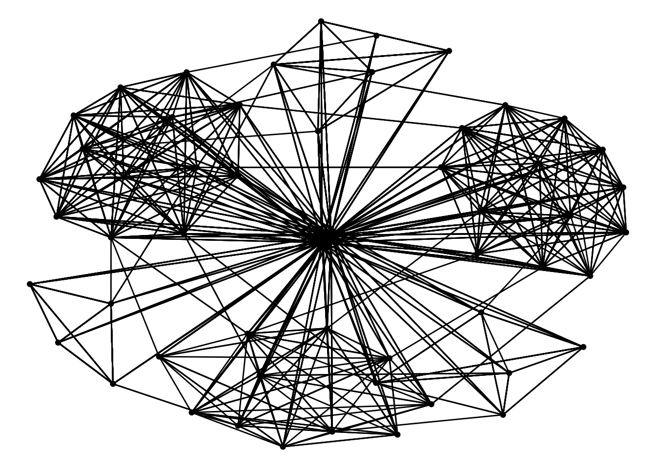
g <- ggraph(GAStech_graph) +
  geom_edge_link(aes(colour = 'grey50')) +
  geom_node_point(aes(colour = 'grey40'))
Using "stress" as default layoutg + theme_graph(background = 'grey10',
text_colour = 'white')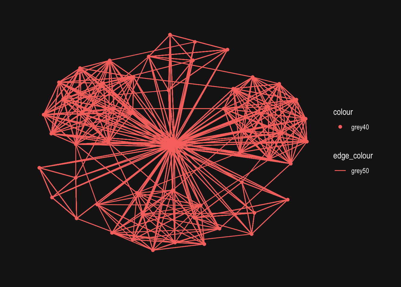
g <- ggraph(GAStech_graph,
            layout = "fr") +
  geom_edge_link(aes()) +
  geom_node_point(aes())

g + theme_graph()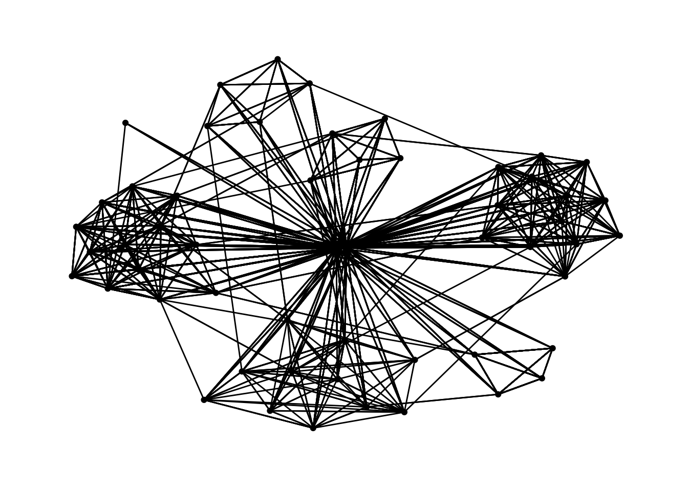
g <- ggraph(GAStech_graph,
            layout = "nicely") +
  geom_edge_link(aes()) +
  geom_node_point(aes(colour = Department,
                      size = 3))

g + theme_graph()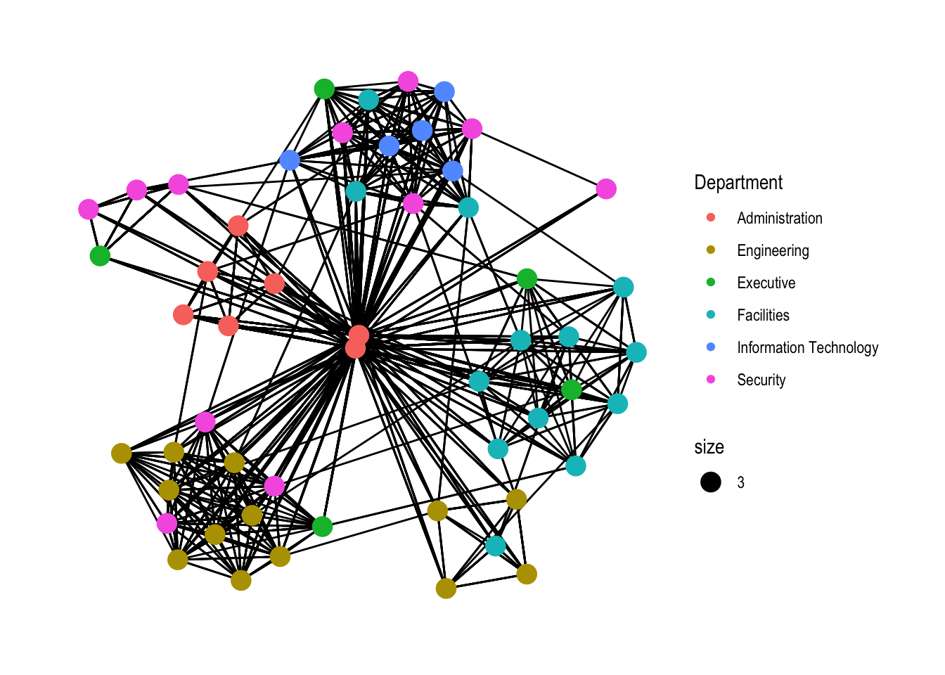
GAStech_edges_aggregated <- GAStech_edges %>%
  left_join(GAStech_nodes, by = c("sourceLabel" = "label")) %>%
  rename(from = id) %>%
  left_join(GAStech_nodes, by = c("targetLabel" = "label")) %>%
  rename(to = id) %>%
  filter(MainSubject == "Work related") %>%
  group_by(from, to) %>%
    summarise(weight = n()) %>%
  filter(from!=to) %>%
  filter(weight > 1) %>%
  ungroup()
`summarise()` has grouped output by 'from'. You can override using the
`.groups` argument.visNetwork(GAStech_nodes,
GAStech_edges_aggregated)visNetwork(GAStech_nodes,
GAStech_edges_aggregated) %>%
visIgraphLayout(layout = "layout_with_fr") GAStech_nodes <- GAStech_nodes %>%
rename(group = Department) visNetwork(GAStech_nodes,
GAStech_edges_aggregated) %>%
visIgraphLayout(layout = "layout_with_fr") %>%
visEdges(arrows = "to",
smooth = list(enabled = TRUE,
type = "curvedCW")) %>%
visOptions(highlightNearest = TRUE,
nodesIdSelection = TRUE) %>%
visLegend() %>%
visLayout(randomSeed = 123)